Introduction
Many forex traders struggle with either a losing strategy or a cyclical one—where gains and losses follow a pattern. However, with the right mathematical tricks and probability-based calculations, you can turn your strategy into a profitable one.
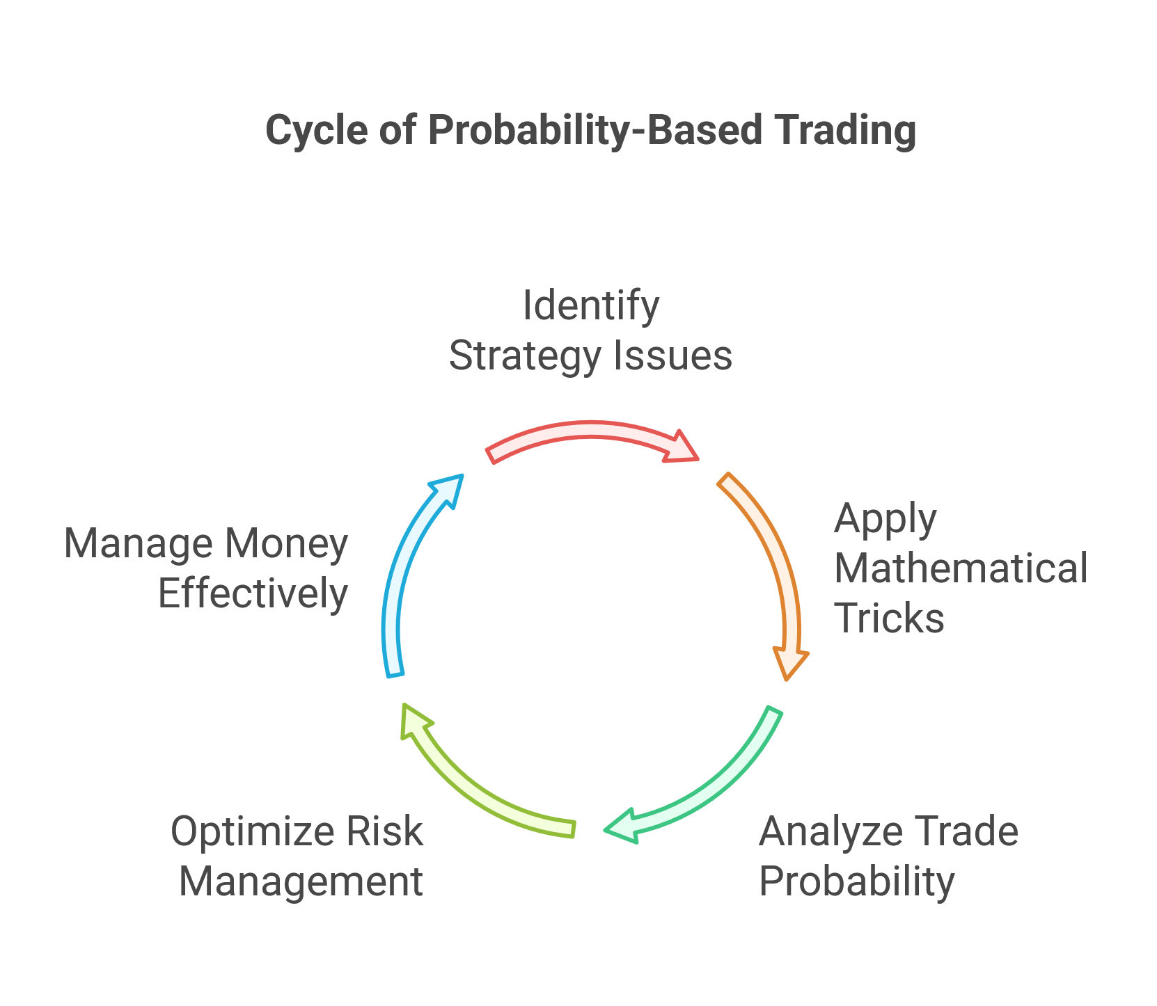
One powerful approach is analyzing the probability of the next move in your trading history. By understanding the likelihood of a trade continuing in the same direction, you can optimize your risk management and money management strategies.
Understanding Trade Probability
Whether you’re a quantitative trader or a manual forex trader, analyzing your past trades can reveal useful probability patterns.
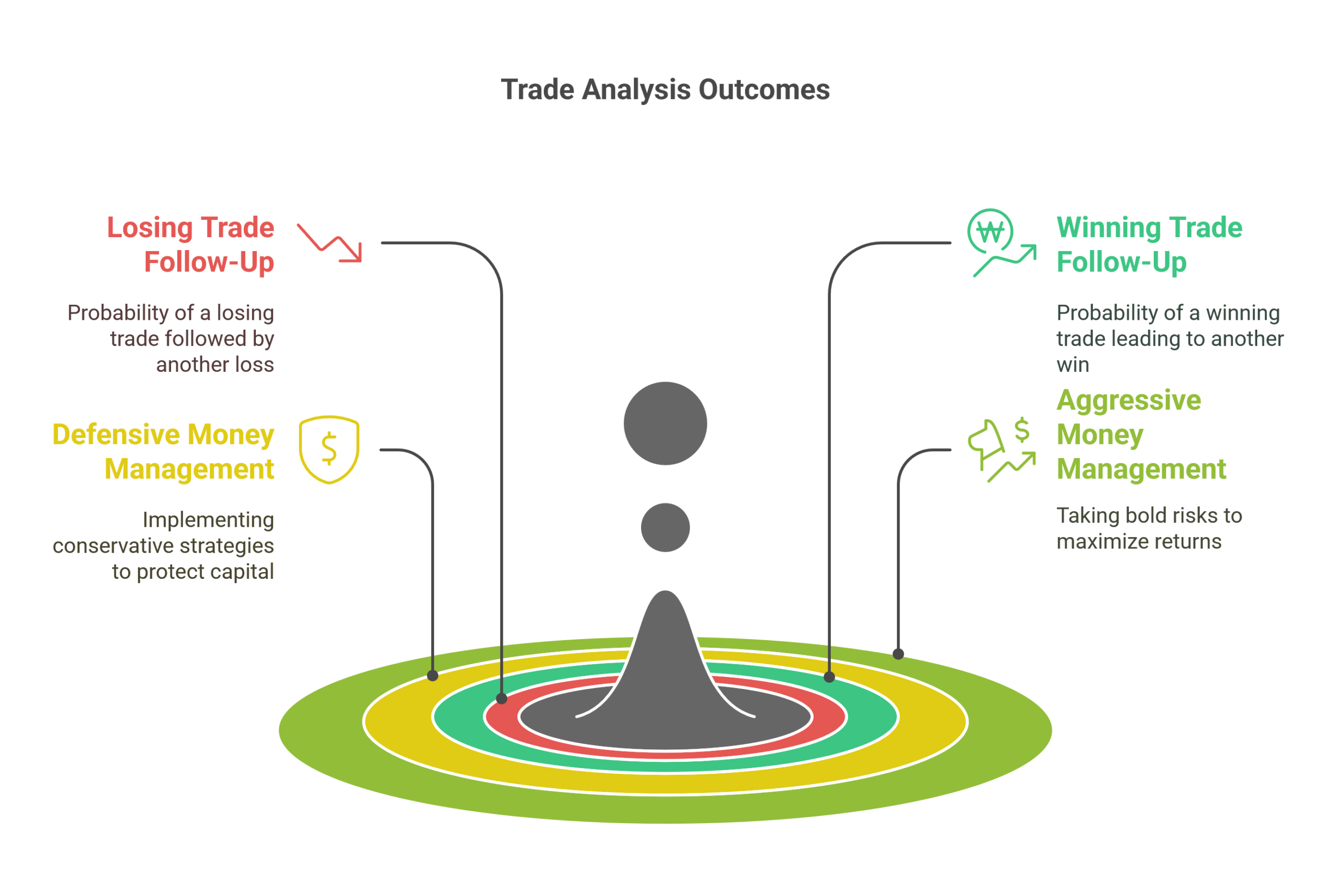
For example, you can assess:
- The probability of a losing trade being followed by another loss.
- The probability of a winning trade leading to another profitable trade.
By leveraging these insights, you can implement defensive or aggressive money management techniques to enhance your overall performance.
Applying Probability to Money Management
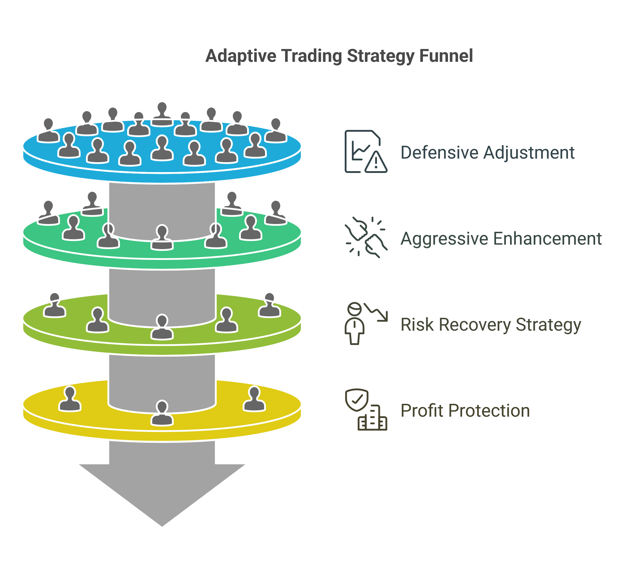
1. Defensive Money Management
If your trade history shows a 60% probability of making a loss after a losing trade, you can reduce your risk by adjusting your trading volume.
Example:
- After a loss, reduce your position size by half to minimize further losses.
- This approach helps preserve capital and avoid consecutive heavy losses.
2. Aggressive Money Management
If your analysis reveals a 60% probability of making a profit after a profitable trade, you can take a more aggressive approach.
Example:
- After a winning trade, increase your trading volume (e.g., double it) to maximize gains.
- This way, you capitalize on winning streaks and boost your profitability.
3. Martingale Strategy (Riskier Approach)
If your trading statement shows that after a loss, there is a 40% probability of making a profit, you can apply a modified Martingale strategy.
Example:
- After a loss, double your trading volume.
- Since there’s a 60% probability of a win after a loss, this approach aims to recover previous losses and secure profits.
4. Reducing Risk After Winning Trades
If your probability analysis shows a 60% likelihood of losing after a profitable trade, you should consider reducing your trade size.
Example:
- After a win, halve your trade volume to protect profits and minimize potential drawdowns.
Final Thoughts
Trading success isn’t just about strategy—it’s about adapting based on probabilities. By analyzing your past trades and applying probability-based money management, you can make more informed decisions and reduce unnecessary risks.
Key Takeaways:
✔ Identify trade probabilities in your historical data.
✔ Adjust your position size based on probability to optimize performance.
✔ Use defensive money management to minimize losses.
✔ Apply aggressive strategies to capitalize on winning streaks.
✔ Consider Martingale cautiously, ensuring probabilities support it.
By incorporating these probability-based adjustments, you can significantly improve your trading strategy and increase long-term profitability.
What is MetaTrader, and how do I use it?
Simple Example in Python :
import numpy as np
import matplotlib
matplotlib.use('QtAgg')
import matplotlib.pyplot as plt
np.random.seed(44)
random_moves = np.random.choice([1, -1], size=199)
prices_fair = np.cumsum(np.insert(random_moves * np.random.uniform(1, 5, size=199), 0, 100))
returns = np.diff(prices_fair)
def defensive_optimize(arr,base=2,step=1.0,max_step=1):
step_moved = 1
first_base = base
for i in range(1,len(arr)):
if arr[i-1] < 0:
arr[i] = arr[i] / base
else:
step_moved = 1
base = first_base
if max_step > 1 and step > 0 and step_moved +1 <= max_step:
print('-Base : ', base)
print('-Moved : ', step_moved)
base += step
step_moved += 1
print('Base : ',base)
print('Moved : ',step_moved)
return arr
def aggressive_optimize(arr,base=2,step=1.0,max_step=1):
step_moved = 1
first_base = base
for i in range(1,len(arr)):
if arr[i-1] > 0:
arr[i] = arr[i] * base
else:
step_moved = 1
base = first_base
if max_step > 1 and step > 0 and step_moved +1 <= max_step:
print('-Base : ', base)
print('-Moved : ', step_moved)
base += step
step_moved += 1
print('Base : ',base)
print('Moved : ',step_moved)
return arr
#------------------
returns_defensive_optimized = defensive_optimize(arr=returns.copy())
returns_aggressive_optimized = aggressive_optimize(arr=returns.copy())
returns_combined_optimize = defensive_optimize(arr=returns.copy())
returns_combined_optimize = aggressive_optimize(arr=returns_combined_optimize)
#------------------
cumsum_returns = np.cumsum(returns)
cumsum_returns_defensive_optimized = np.cumsum(returns_defensive_optimized)
cumsum_returns_aggressive_optimized = np.cumsum(returns_aggressive_optimized)
cumsum_returns_combined_optimize = np.cumsum(returns_combined_optimize)
#------------------
moves = np.where(returns > 0, 1, -1)
up_moves = np.sum(moves[:-1] == 1)
down_moves = np.sum(moves[:-1] == -1)
up_after_up = np.sum((moves[:-1] == 1) & (moves[1:] == 1))
down_after_down = np.sum((moves[:-1] == -1) & (moves[1:] == -1))
# Compute probabilities
p_up_given_up = up_after_up / up_moves if up_moves > 0 else 0
p_down_given_down = down_after_down / down_moves if down_moves > 0 else 0
# Print results
print(f"P(Up | Up) = {p_up_given_up:.2%}")
print(f"P(Down | Down) = {p_down_given_down:.2%}")
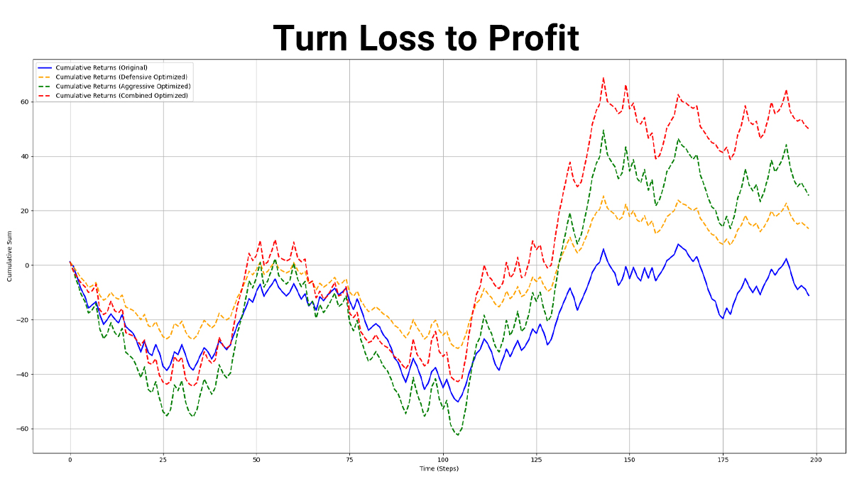
plt.figure(figsize=(12, 6))
plt.plot(cumsum_returns, label="Cumulative Returns (Original)", color="blue", linewidth=2)
plt.plot(cumsum_returns_defensive_optimized, label="Cumulative Returns (Defensive Optimized)", color="orange", linewidth=2, linestyle="dashed")
plt.plot(cumsum_returns_aggressive_optimized, label="Cumulative Returns (Aggressive Optimized)", color="green", linewidth=2, linestyle="dashed")
plt.plot(cumsum_returns_combined_optimize, label="Cumulative Returns (Combined Optimized)", color="red", linewidth=2, linestyle="dashed")
plt.xlabel("Time (Steps)")
plt.ylabel("Cumulative Sum")
plt.title("Comparison of Cumulative Returns: Original vs Optimized")
plt.legend()
plt.grid(True)
plt.show()


